Explanation Shift Detector
This tutorial enables to measures of explanation shifts as way to detect model shifting behaviour. As we have discussed inthe paper, it can provide more insights than measures of the input distribution and prediction shift when monitoring machine learning models.
In this section we provide examples of usage over two different datasets. The first one the shift is generated synthetically and in the second one is a natural shift.
Note
This project is under active development.
Breast Cancer Dataset
Importing libraries
import numpy as np
from sklearn.datasets import make_blobs
from xgboost import XGBRegressor
from sklearn.linear_model import LogisticRegression
from skshift import ExplanationShiftDetector
from sklearn.model_selection import train_test_split
Generate synthetic ID and OOD data.
# Real World Example
from sklearn import datasets

# import some data to play with
dataset = datasets.load_breast_cancer()
X = dataset.data[:, :5]
y = dataset.target
X_tr, X_te, y_tr, y_te = train_test_split(X, y, test_size=0.5, random_state=0)

X_ood = X.copy()
X_ood[:, 0] = X_ood[:, 0] + 3
# Split in train and test
X_ood_tr, X_ood_te, y_ood_tr, y_ood_te = train_test_split(
    X_ood, y, test_size=0.5, random_state=0
)
# Concatenate for new dataset
X_new = np.concatenate([X_te, X_ood_te])
y_new = np.concatenate([np.zeros_like(y_te), np.ones_like(y_ood_te)])
Fit Explanation Shift Detector whith model and detector being an xgboost
detector = ExplanationShiftDetector(model=XGBClassifier(), gmodel=XGBClassifier())

detector.fit_pipeline(X_tr, y_tr, X_te, X_ood_tr)

roc_auc_score(y_new,detector.predict_proba(X_new)[:,1])
# 0.93
If the AUC is above 0.5 then we can expect and change on the model predictions. Now we can proceed to explain how the model changed between test and OOD data.
The intuition of this explanations is what are the features driving OOD model behaviour?
# Explaining the change of the model
import shap
explainer = shap.Explainer(detector.detector, masker=detector.get_explanations(X))
shap_values = explainer(detector.get_explanations(X_ood_te))
shap.waterfall_plot(shap_values[0])
shap.plots.bar(shap_values)

As the model used is a XGBoost we can see that even if we shift a univariate feature the model detects correlation with other features that are modifying model behaviour
Folktables: US Income Dataset
In this case we use the US Income dataset. The dataset is available in the Folktables repository.
We generate a geopolitical shift by training on California data and evaluating on other states.
from folktables import ACSDataSource, ACSIncome
import pandas as pd

data_source = ACSDataSource(survey_year="2018", horizon="1-Year", survey="person")
ca_data = data_source.get_data(states=["CA"], download=True)
pr_data = data_source.get_data(states=["PR"], download=True)
ca_features, ca_labels, _ = ACSIncome.df_to_pandas(ca_data)
pr_features, pr_labels, _ = ACSIncome.df_to_pandas(pr_data)

# Split ID data and OOD train and test data
X_tr, X_te, y_tr, y_te = train_test_split(
    ca_features, ca_labels, test_size=0.5, random_state=0
)
X_ood_tr, X_ood_te, y_ood_tr, y_ood_te = train_test_split(
    pr_features, pr_labels, test_size=0.5, random_state=0
)
X_new = pd.concat([X_te, X_ood_te])
y_new = np.concatenate([np.zeros_like(y_te), np.ones_like(y_ood_te)])

# Fit the model
model = XGBClassifier().fit(X_tr, y_tr)
The model is trained on CA data, and evaluated on data with OOD
detector = ExplanationShiftDetector(model=model, gmodel=XGBClassifier())
detector.fit_detector(X_te, X_ood_te)
roc_auc_score(y_new, detector.predict_proba(X_new)[:, 1])
# 0.96
The AUC is high which means that the model is changing. We can now proceed to inspect the model behaviour change.
explainer = shap.Explainer(detector.detector)
shap_values = explainer(detector.get_explanations(X_new))
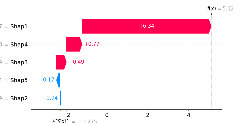
# Local Explanations for instance 0
shap.waterfall_plot(shap_values[0])
# Global Explanations
fig = shap.plots.bar(shap_values)
We proceed to the explanations of the Explanation Shift Detector

Above local explanations, below global explanations

Now we can proceed to do the same with a less OOD data, the US Income from the state of Michigan.
# Now if we choose a differet OOD data
tx_data = data_source.get_data(states=["TX"], download=True)
tx_features, tx_labels, _ = ACSIncome.df_to_pandas(tx_data)

# Split data
X_tr, X_te, y_tr, y_te = train_test_split(
    ca_features, ca_labels, test_size=0.5, random_state=0
)
X_ood_tr, X_ood_te, y_ood_tr, y_ood_te = train_test_split(
    tx_features, tx_labels, test_size=0.5, random_state=0
)
X_new = pd.concat([X_te, X_ood_te])
y_new = np.concatenate([np.zeros_like(y_te), np.ones_like(y_ood_te)])
detector = ExplanationShiftDetector(model=model, gmodel=XGBClassifier())

detector.fit_detector(X_te, X_ood_te)
print(roc_auc_score(y_new, detector.predict_proba(X_new)[:, 1]))
# 0.82
We can see how the AUC of the model is different. And proceed to inspect the model behaviour change. The local explanations:

The global explanations:
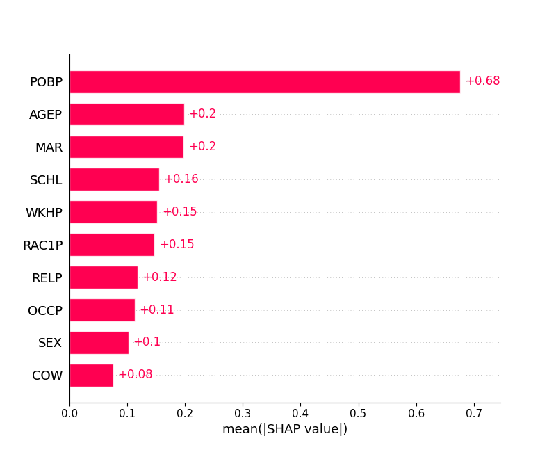
We can see how the model behaviour is changing between the two states. By comparing the images we can see that the feature attributions to the reasons of the OOD explanation are distinct between the data two states.